A successful interferometric setup requires that the SPPDI and the optical system under test be mounted in stable optical mounts with precision angle and linear motion adjusters. A low vibration environment with small temperature variations is very helpful.
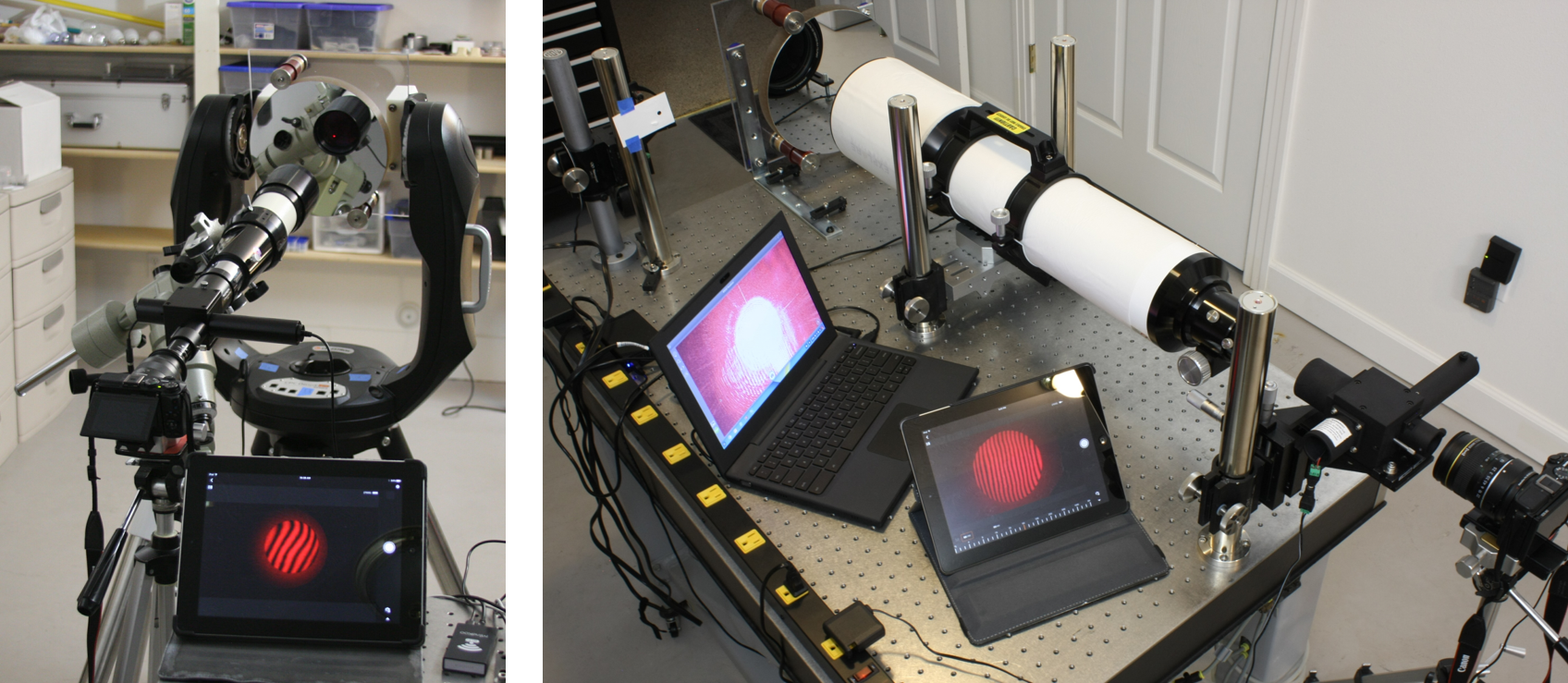 A 2-inch diameter Telescope Adapter is provided with the SPPDI to facilitate direct attachment of the SPPDI to the 2″ eyepiece holder typically provided with higher-end commercial telescopes. Such an arrangement is shown in the photo on the left.
For larger refractors, such as the 5″ refractor shown in the photo on the right, the prime (far-field) focal plane for the telescope objective is so far distant from the rear of the scope that two extension tubes are required in order to position the SPPDI at prime focus. This does not lend itself to precise positioning of the SPPDI with respect to the optical axis of the objective lens. Use of the diagonal mirror eyepiece holder typically provided with these telescopes would enable prime focus to be reached without the use of extenders, but could compound the errors in the objective lens with errors in the diagonal mirror.
So, to avoid these complications, the SPPDI is mounted separately on a three-axis translation stage setup as shown in the photo on the right. This requires that the telescope first be brought into autocollimation with the “optical flat” (high precision flat mirror) used for double-pass interferometry. This is easily accomplished by means of a low cost laser alignment tool typically sold for the purpose of aligning the primary mirror in Newtonian type telescopes. Then the SPPDI is positioned along the x, y, and z axes by means of the translation stages. For reflector type telescopes with low-profile focusers, the SPPDI may be easily positioned at prime focus. Note that the SPPDI pinhole aperture is located at a depth of about 32.5 mm inside the SPPDI enclosure.
As the telescope focal length increases, isolation from ambient vibration becomes increasingly difficult. It is very helpful to have all equipment co-located on a stable platform, such as on an optical table like the one shown in the photo on the right.
The 10″ optical flat seen in the photo above left is mounted in a fork mount obtained by disassembling a large (11″ aperture) commercial Schmidt-Cassegrain type telescope. The optical tube assembly was replaced with a purpose-built saddle capable of supporting a 12-inch diameter optical flat. The electronic slow motion control associated with the fork mount is used to bring the telescope under test into near autocollimation against the optical flat. Final precision alignment is achieved by means of a set of three 1/4×20 jack screws mounted on the ends of three long lever arms which support and raise and lower the tripod feet.
Measurement Methods and Use-Cases
1.) CoC: Center of Curvature.
This use-case applies to measurement of concave reflective optics, such as spherical or parabolic mirrors that are measured at their CoC. Mirrors with focal ratios (“speeds”) as fast as f/2 (i.e., f/4 at CoC) may be measured directly by the SPPDI without any ancillary optics interposed between the test article and the SPPDI. Test beams outside the “normal” range of f/4 to f/12 may be measured with the use of external beam forming optics as described below.
Two very “fast” (f/0.5 and f/1.27) 2″ diameter high precision (<1/10th wave) fused silica concave spherical mirrors are available from Kerry Optical Systems for use in measuring and compensating for aberrations in the SPPDI internal optics and any external beam forming optics that may be required. An error-compensating wavefront is obtained with the aid of the reference mirror, at the same focal ratio as for the test article, which is subtracted from the wavefront of the test article, to yield a high accuracy wavefront map for the test article.
2.) DPAC: Double-pass At Autocollimation.
This use-case is applicable for measuring either transmissive optics or reflective optics or optical systems that are optimized for observation or recording of remote objects. This use-case requires the use of an accurate optical flat of sufficient size to reflect the collimated output beam back through the test article.
As mentioned in the CoC use-case, measurements of test beams with focal ratios outside the SPPDI “normal range” will require the use of external beam forming optics. Calibration optics must be used to remove instrumental errors as discussed in the CoC use-case.
3.) PSI (Phase Shift Interferometry)
PSI is easily done with the SPPDI. A rotatable QWP (quarter-wave plate optimized for 650 nm) is installed in the external beam path in front of the camera lens rotatable linear polarizer. The SPPDI internal polarizers must be rotated to a condition to produce orthogonally polarized signal and reference beams. The external QWP and camera lens polarizer are rotated independently to achieve a balanced fringe contrast over the full rotational range of the camera polarizer. After this balance is achieve, the internal SPPDI polarizers and QWP remain fixed while the camera polarizer is rotated through the full 0° to 180° rotational range for phase shifting.
4.) Beam Forming Optics
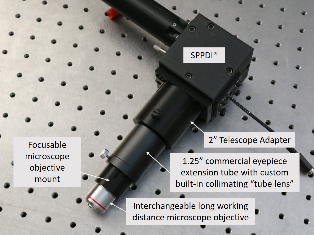 The SPPDI by itself is physically limited to measuring converging incident beams that lie in the f/4 to f/12 “normal” range.” So, beam forming optics must be used when the incident test beam lies outside the “normal” range. This figure shows the components that comprise the Kerry Optical Systems Tube Lens Collimator in a so-called “Transmission Sphere” setup for measuring optical systems that have focal ratios that lie outside the SPPDI f/4 – f/12 “normal” range.
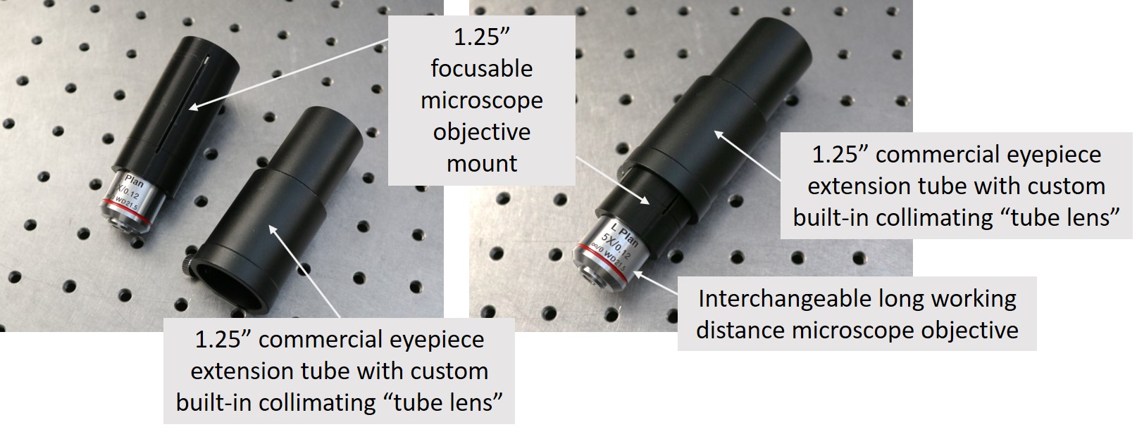
A “Transmission Sphere” system comprises three parts, all of which can be purchased separately from Kerry Optical Systems: (1) a collimating “tube lens” mounted in the small (1.25″ OD) end of the supplied COTS eyepiece extender; (2) a compression mount that fits in the eyepiece end of the COTS eyepiece extender; and (3) a user-supplied refocusing lens for matching the focal ratio requirements of the system under test. The “tube lens” receives an f/8 portion of the diverging beam from the SPPDI and collimates the beam to a diameter of about 8 or 9 mm. This diameter just overfills the rear aperture (typically 8 or 9 mm) of interchangeable microscope objectives that screw into the RMS threaded end of the compression mount. Alternatively, refocusing lenses other than microscope objectives may be used to produce output beams which match the focal ratio requirements of the specific optical system under test. The user should be careful to avoid using more than an 8 or 9 mm diameter portion of the collimated beam produced by the tube lens.
IMPORTANT: The Transmission Sphere setup described above should not be used for measuring fast aspheric optics at their CoC. Geometrical aberrations or large optical errors in the test beam introduce retrace errors in the Transmission Sphere optics that cannot be adequately predicted or compensated for.
IMPORTANT: It should be noted that a Transmission Sphere setup will produce a relayed image of the test article that will appear close to the SPPDI main port. This will require the user to attach a 9x or 10x close-up lens to the camera lens to produce a properly focused image of the test article.
5.) Correction Wavefront
The Transmission Sphere setup described here may be used in combination with either our precision reference mirror or our precision Random Ball Test Kit, to produce a correction wavefront, which can then be subtracted from the wavefront obtained for the test article. This process allows removal of the errors associated with the Transmission Sphere as well as the SPPDI.
The interferogram and associated wavefront for the test article should be obtained first, with a DFTFringe outline that is suitable for the test article. This same outline must then be used in obtaining the correction wavefront using the calibration optics.
5.) Selecting a Suitable Camera for Recording Interference Fringes
There are several things to consider. When you test any optical system with the SPPDI, you must position the internal pinhole of the SPPDI at the focus of the optical system you are testing. The SPPDI pinhole lies 32.5 mm deep inside the SPPDI front face (side facing the test object). The SPPDI does not modify the f/# of the system you are testing. So, the beam exiting the SPPDI will have the same f/# as the beam entering the SPPDI. So, in order to not vignette the beam exiting the SPPDI with your camera lens, you must choose a camera lens with an aperture that can accept the expanding beam without vignetting the beam, i.e., before the beam footprint grows too large for the pupil of your camera lens.
You can assume that the beam exiting the exit ports of the SPPDI will appear to diverge from a point that lies around 1.5″ deep inside the SPPDI body. So, by the time the beam exits the SPPDI, it is already fairly large in diameter, depending on the focal ratio of the beam entering the SPPDI. “Faster” test articles will produce beams that grow faster as they exit the SPPDI. And also, you will need to avoid bumping into the SPPDI fringe adjustment handles with your camera lens. So, altogether, you should plan to accommodate a minimum standoff distance to your camera lens pupil of something like 3.5″.
Faster camera lenses will provide a larger standoff distance, before you begin to vignette the beam with your camera lens. As an example, at the minimum standoff distance of 3.5″, an f/4 (“fastest” focal ratio that can be accommodated by the SPPDI) beam from a test article will have grown to a diameter of 3.5″/4 = 0.88″. An 85 mm f/1.2 lens has a pupil size of 85 mm / 1.2 = 71 mm, or about 2.8″, so you should not have any issues with vignetting the 0.88″ diameter beam.
The next thing to consider is the required size of the camera sensor. If you are going to use an 85 mm focal length camera lens, and you are going to measure an f/4 test beam, the beam footprint on the camera sensor will be 85 mm / 4 = 21.5 mm. This image size will overfill an APS-C size sensor which has dimensions of 22.3 mm x 14.9 mm, but will work OK with a full frame digital camera sensor which has dimension of 36 mm x 24 mm.
As another example, a Micro4/3 sensor has dimensions of 18 x 13.5mm. So, a 42.5mm f.l. lens will produce an image of an f/4 test article that will be 42.5mm / 4 = 10.6 mm in diameter. This image size will fit well on this sensor size. As a general rule, you should use the longest focal length, largest aperture lens you can, while still getting an image that does not overfill the size of the camera sensor.
6.) Wavefront “Sense”
An interferogram is a topographic map of a wavefront. Just as in reading a topographic map of a mountain, it is often difficult to know whether traversing the map from fringe to fringe leads uphill or downhill. For optical interferometry, sophisticated and expensive optics can be introduced in the beam path that eliminates the confusion. Fortunately, there is a very simple method for determining the wavefront “sense” which does not require expensive add-on optics. The method involves defocusing the wavefront, and observing the algebraic sign of the Zernike Z3 Defocus term, as displayed by DFTFringe. If the interferometer has moved closer to the test article, the algebraic sign of the Z3 term should become more negative, but all other Zernike terms should remain approximately the same. If the Z3 term becomes more positive, then the DFTFringe “Invert” function should be launched to invert the defocused wavefront. If the Z8 terms of the defocused and non-defocused wavefronts no longer have the same algebraic sign, then the non-defocused wavefront should be inverted.
![]()